Quadratic Regression

 Quadratic regression is a statistical method used to model a relationship between variables with a parabolic best-fit curve, rather than a straight line. It's ideal when the data relationship appears curvilinear. The goal is to fit a quadratic equation  

y=ax^2+bx+c

$y=a{x}^2+bx+c$

to the observed data, providing a nuanced model of the relationship. Contrary to historical or biological connotations, "regression" in this mathematical context refers to advancing our understanding of complex relationships among variables, particularly when data follows a curvilinear pattern.

Working with quadratic regression

These calculations can become quite complex and tedious. We have just gone over a few very detailed formulas, but the truth is that we can handle these calculations with a graphing calculator. This saves us from having to go through so many steps -- but we still must understand the core concepts at play.

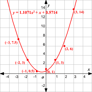
Let's try a practice problem that includes quadratic regression. Consider the following set of data: {(-3,7.5),(-2,3),(-1,0.5),(0,1)(1,3),(2,6),(3,14)}

$\left\{\left(-3,7.5\right),\left(-2,3\right),\left(-1,0.5\right),\left(0,1\right),\left(1,3\right),\left(2,6\right),\left(3,14\right)\right\}$

Can we determine the quadratic regression for this set?

Our first step is to enter our x-coordinates and y-coordinates into our graphing calculator. We can then carry out our operation for a quadratic equation. This will give us the equation of the parabola that best approximates the points: y=1.1071x^2+x+0.5714

$y=1.1071x^2+x+0.5714$

Great! Now all we need to do is plot our graph. We should be left with something like this:

We also know that our relative predictive power ( $R^2$ ) is 0.9942. That's pretty accurate -- and it tells us that our calculations for quadratic regression worked!

##################################################################################

import numpy as np

import matplotlib.pyplot as plt

import pandas as pd

from sklearn.linear_model import LinearRegression

from sklearn.preprocessing import PolynomialFeatures

# Load data from CSV file

data = pd.read_csv('C:/Users/srinu/Downloads/3-4_CSM_ML/Dataset/data1.csv')  # Replace 'data.csv' with your file name

# Extract the independent (X) and dependent (Y) variables

x = data['X'].values.reshape(-1, 1)

y = data['Y'].values

# Transform the data to include x^2

poly = PolynomialFeatures(degree=2)

x_poly = poly.fit_transform(x)

# Fit the model

model = LinearRegression()

model.fit(x_poly, y)

# Make predictions

y_pred = model.predict(x_poly)

# Plotting the results

plt.scatter(x, y, color='blue', label='Original data')

plt.plot(x, y_pred, color='red', label='Quadratic regression')

plt.xlabel('X')

plt.ylabel('Y')

plt.title('Quadratic Regression')

plt.legend()

plt.show()

Data Set 

X,Y

1,1

2,4

3,9

4,16

5,25

6,36

7,49

8,64

9,81

Other Data set

# importing packages and modules 

import pandas as pd 

import numpy as np 

import matplotlib.pyplot as plt 

import seaborn as sns 

from sklearn.metrics import r2_score 

import scipy.stats as stats 

dataset = pd.read_csv('ball.csv') 

sns.scatterplot(data=dataset, x='time', 

y='height', hue='time') 

plt.title('time vs height of the ball') 

plt.xlabel('time') 

plt.ylabel('height') 

plt.show() 

# degree 2 polynomial fit or quadratic fit 

model = np.poly1d(np.polyfit(dataset['time'], 

dataset['height'], 2)) 

# polynomial line visualization 

polyline = np.linspace(0, 10, 100) 

plt.scatter(dataset['time'], dataset['height']) 

plt.plot(polyline, model(polyline)) 

plt.show() 

print(model) 

# r square metric 

print(r2_score(dataset['height'], 

model(dataset['time'])))